二阶偏微分方程(一) #拉普拉斯算子

　　如果只是解微分方程，略显枯燥。能给出具体场景应用，就有意思了。
SIGGRAPH 2003 出现一篇论文

图像泊松融合 《Poisson Image Editing》(Christopher J. Tralie, Ph.D.)，

可以无缝衔接两张图。

OpenCV 3 实现该功能后取名为 Seamless Cloning。
https://docs.opencv.org/4.x/df/da0/group__photo__clone.html

这里介绍了关于泊松方程在图像和形状相关的应用[8]，
对图像的编辑，给出了5篇 SIGGRAPH 论文，可结合理论深入学习。

• Poisson Image Editing
• Seamless Image Stitching in the Gradient Domain
• Interactive Digital Photomontage
• Drag-and-Drop Pasting
• Efficient Gradient-Domain Compositing Using Quadtrees

　　无缝融合图像是以源图像块内的梯度场为向导，将融合边界上目标场景和源图像的差异平滑地扩散到融合图像块中，该操作使得，融合后的图像块能够无缝地融合到目标场景中，并且其色调和光照可以与目标场景保持一致。

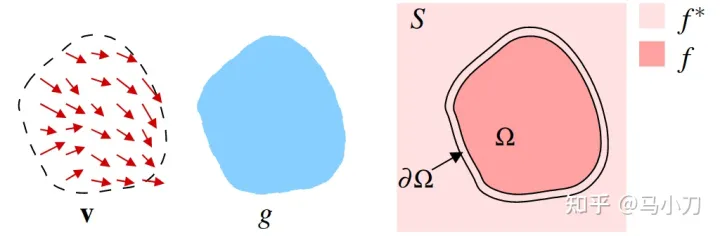
以v为梯度场，f*的接壤处为边界Ω，可参考梯度场g，求解未知函数f

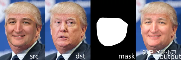
seamlessClone(src, dst, mask, center, output, NORMAL_CLONE);

参考

1. ^以拉普拉斯命名的事物 https://en.wikipedia.org/wiki/List_of_things_named_after_Pierre-Simon_Laplace
2. ^拉普拉斯方程 https://en.wikipedia.org/wiki/Laplace%27s_equation
3. ^是公式都会追求短而美 https://www.zhihu.com/question/26992291/answer/1448275421
4. ^可分离变量的偏微分方程 https://en.wikipedia.org/wiki/Separable_partial_differential_equation
5. ^解二阶常系数齐次线性微分方程 https://en.wikipedia.org/wiki/Linear_differential_equation#Second-order_case
6. ^唯一性定理 https://en.wikipedia.org/wiki/Uniqueness_theorem_for_Poisson%27s_equation
7. ^反函数及其微分 https://en.wikipedia.org/wiki/Inverse_functions_and_differentiation
8. ^The Poisson Equation in Image & Shape Processing https://www.cs.jhu.edu/~misha/Fall07/

编辑于 2023-04-22 19:33・IP 属地中国香港

《Poisson Image Editing》论文理解与复现

2023年4月9日 本报告的主要内容是阅读《Poisson Image Editing》论文之后对原理进行理解并利用python复现论文中的每个功能。 2. 引言 图像融合是图像处理的一个基本问题,目的是将源图像中一个物体…

betheme.net/yidongkaifa/42…html

Poisson Image Editing

https://zhuanlan.zhihu.com/p/355055346

本文使用 Zhihu On VSCode 创作并发布

1. Poisson Image Seamless Cloning-2003

• 论文传送门Poisson Image Editing

这类文章非常简单： Reconstruct a funtion from its gradients via Poisson Equation。值域的直接Cloning有接缝，那么间接的在微分坐标域内Cloning, 再求解Poisson方程即可。 未知变量为mask指定的内部区域，Dirichlet Boundary Condition为宿主图像上mask指定以外的部分。当然也有经典的Poisson Mesh Editing, 也是同样的套路。Poisson Image Cloning是直接对像素值建微分方程的，而图像处理中则有另外一类操作是对图像建一个Proxy, 如经典的2D图像动画等等。

<code>def poisson_cloning(src, dst, mask):
    src_delta = cv2.Laplacian(src.astype(np.float32), cv2.CV_32FC1, 1)
    dst_delta = cv2.Laplacian(dst.astype(np.float32), cv2.CV_32FC1, 1)
    delta = src_delta*0.8+0.2*dst_delta

    h, w = mask.shape 
    num_pxls = h * w
    laplacian = sps.eye(num_pxls, dtype='float64', format="dok")
    for i in range(1, h-1):
        for j in range(1, w-1):
            if mask[i, j]: 
                laplacian[i*w+j, i*w+j] = -4
                laplacian[i*w+j, i*w+(j-1)] = 1
                laplacian[i*w+j, (i-1)*w+j] = 1 
                laplacian[i*w+j, i*w+(j+1)] = 1 
                laplacian[i*w+j, (i+1)*w+j] = 1

    delta[np.where(mask == 0)] = dst[np.where(mask == 0)]
    x = spsolve(laplacian.tocsr(), delta.flatten())
    x = np.clip(x, 0, 255)
    return x.reshape(dst.shape).astype(np.uint8)

2. Poisson Image Matting-2004

• 论文传送门Poisson Matting
• 
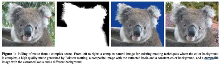  Image这个文章其实现在看来，理论非常牵强效果也不好，还是经典的Closed Form Matting更值得学习。 这种Trimap的羽化问题，远没有2010年的何凯明的Guide Filtering做得好。文章的一作Jian Sun是Guide Filtering的二作，学生做好了。孙老师认为Alpha Matte的边界一定会是输入的图像边界的一个子集, 在图像的平滑区域，微分坐标接近为零，在Alpha Matte的边界处的微分坐标和输入图像的微分坐标一致。然后Alpha Matte至少具有双边界， 固定边界求解Poisson方程即可。

def sparse_matrix_solver(alpha, b, mask):
    h, w = mask.shape 
    num_pxls = h * w
    laplacian = sps.eye(num_pxls, dtype='float64', format="dok")
    for i in range(1, h-1):
        for j in range(1, w-1):
            if mask[i, j]: 
                laplacian[i*w+j, i*w+j] = -4
                laplacian[i*w+j, i*w+(j-1)] = 1
                laplacian[i*w+j, (i-1)*w+j] = 1 
                laplacian[i*w+j, i*w+(j+1)] = 1 
                laplacian[i*w+j, (i+1)*w+j] = 1

    b[np.where(mask == 0)] = alpha[np.where(mask == 0)]
    alpha = spsolve(laplacian.tocsr(), b.flatten())
    return alpha.reshape(mask.shape)


def poisson_matte(gray_img, trimap):
    fg, bg = (trimap == 255), (trimap == 0)
    unknown = True ^ np.logical_or(fg, bg)
    Estimate_alpha = fg + 0.5 * unknown
    
    gray_bg, gray_fg = (gray_img*bg).astype(np.uint8), (gray_img*fg).astype(np.uint8)

    fg_approx = cv2.inpaint(gray_fg, (bg+unknown).astype(np.uint8)*255, 3, cv2.INPAINT_TELEA)*(fg+unknown)
    bg_approx = cv2.inpaint(gray_bg, (fg+unknown).astype(np.uint8)*255, 3, cv2.INPAINT_TELEA)*(bg+unknown)

    bg_approx, fg_approx = bg_approx.astype(np.float32), fg_approx.astype(np.float32)

    diff_approx = scipy.ndimage.filters.gaussian_filter(fg_approx - bg_approx, 0.9)+1e-4

    dy, dx = np.gradient(gray_img)
    d2y, _ = np.gradient(dy/diff_approx)
    _, d2x = np.gradient(dx/diff_approx)
    b = d2y + d2x

    New_Alpha = sparse_matrix_solver(Estimate_alpha, b, unknown)
    New_Alpha = np.clip(New_Alpha, 0, 1)

    return New_Alpha